
Data Cleaning and Exploration, The Movie
(Go to the READ.ME of this repository for the entire write-up.)
I collected quite a bit of data: 43837 separate movies. The actual cleaning of the data was as tedious and dry as the following paragraphs.
len(df)
43837
import imdb
import warnings
warnings.simplefilter("ignore")
import re
import pandas as pd
import numpy as np
import ast
from datetime import datetime, timedelta
from sklearn.feature_extraction.text import CountVectorizer

import matplotlib.pyplot as plt
import seaborn as sns

%matplotlib inline
Lost of the data came in lists, such as a list of the first four actors in a film. I had to go through and strip all members of the lists, as well as join lists on pipes to later be separated by my count vectorizer. I wrote a bunch of functions to clean the data, even a few I didn’t need. This functions did thing like turn data to floats or create new columns of data.
def release_to_datetime(n):
    if type(n) == str:
        n = n.replace(' Nov ', '-11-').replace(' Jun ', '-6-').replace(' Aug ', '-8-').replace(' Dec ', '-12-')
        n = n.replace(' Oct ', '-10-').replace(' Jan ', '-1-').replace(' Feb ', '-2-').replace(' Mar ', '-3-')
        n = n.replace(' Apr ', '-4-').replace(' May ', '-5-').replace(' Jul ', '-7-').replace(' Sep ', '-9-')
        n = datetime.strptime(n, '%d-%m-%Y').date()
        return n
    else:
        return n

def delta_release(n):
    y2k = datetime.strptime('01-01-2000', '%d-%m-%Y').date()
    try:
        m = y2k - n
        return m.days
    except:
        return np.nan

def pull_month(n):
    try:
        return n.month
    except:
        return np.nan

def pull_day(n):
    try:
        return n.day
    except:
        return np.nan

def runtime_to_float(x):
    try:
        return float(x)
    except:
        return np.nan

def boxoffice_to_float(x):
    try:
        return float(x.replace(',',"").replace("$",""))
    except:
        return np.nan

def RT_pull_out(entry):
    for m in entry:
        if m['Source'] == 'Rotten Tomatoes':
            n = (m['Value'].replace('%', ''))
            return(int(n))
        else:
            return(np.nan)

def evan_train_test_df_cvec_capstone(train, test, min_df):
    min_df = min_df
    dummy_list_train = []
    dummy_list_test = []
    for x in train.columns:
        cvec = CountVectorizer(binary=True,
                               tokenizer=(lambda m: m.split('|') ),
                               min_df = min_df,
                               stop_words = 'english',
                               strip_accents='unicode')
        cvec.fit(train['{}'.format(x)])
        lonely_matrix_train = cvec.transform(train['{}'.format(x)])
        lonely_matrix_test = cvec.transform(test['{}'.format(x)])
        df_train = pd.DataFrame(lonely_matrix_train.todense(), columns=cvec.get_feature_names())
        df_test = pd.DataFrame(lonely_matrix_test.todense(), columns=cvec.get_feature_names())
        dummy_list_train.append(df_train)
        dummy_list_test.append(df_test)
    dummied_df_train = pd.concat(dummy_list_train, axis=1)
    dummied_df_test = pd.concat(dummy_list_test, axis=1)
    return dummied_df_train, dummied_df_test

def movie_split_and_join(train, test, func, min_df=1):
    train_obj = train.select_dtypes(include=[np.object_])
    train_num = train.select_dtypes(include=[np.number, np.bool_])
    test_obj = test.select_dtypes(include=[np.object_])
    test_num = test.select_dtypes(include=[np.number, np.bool_])
    train_obj_dums, test_obj_dums = func(train_obj, test_obj, min_df)
    train_obj_dums.reset_index(drop=True, inplace=True)
    test_obj_dums.reset_index(drop=True, inplace=True)
    train_num.reset_index(drop=True, inplace=True)
    test_num.reset_index(drop=True, inplace=True)
    final_train = pd.concat([train_num, train_obj_dums], axis=1)
    final_test = pd.concat([test_num, test_obj_dums], axis=1)
    return final_train, final_test

def strip_list(column):
    for n in column:
        for m in range(len(n)):
            n[m] = n[m].strip()
    return column

def put_in_avgs(train, test, df):
    ind = 0
    for n in train.columns:
        for m in list(zip(df.name, df.avgscore)):
            if n == m[0]:
                train[n] *= m[1]
            ind += 1
            if ind % 10000 == 0:
                print(ind)
    ind = 0
    for n in test.columns:
        for m in list(zip(df.name, df.avgscore)):
            if n == m[0]:
                test[n] *= m[1]
            ind += 1
            if ind % 10000 == 0:
                print(ind)
    print(train.shape)
    print(test.shape)
    return train, test

def single_column_cvec(train, test, min_df):
    cvec = CountVectorizer(binary=True,
                                   tokenizer=(lambda m: m.split('|') ),
                                   min_df = min_df,
                                   stop_words = 'english',
                                   strip_accents='unicode')
    cvec.fit(train)
    lonely_matrix_train = cvec.transform(train)
    lonely_matrix_test = cvec.transform(test)
    new_train = pd.DataFrame(lonely_matrix_train.todense(), columns=cvec.get_feature_names())
    new_test = pd.DataFrame(lonely_matrix_test.todense(), columns=cvec.get_feature_names())
    return new_train, new_test
df = pd.read_csv("new_all_my_movies_final.csv", converters={"Actors": ast.literal_eval,
                                                        "Director": ast.literal_eval,
                                                        "Genre": ast.literal_eval,
                                                        "RTRating": ast.literal_eval,
                                                        "Writer": ast.literal_eval,
                                                        "Year": ast.literal_eval})
This following cell contains remnants from what I’ll call “The Actor Average Debacle” later on in the presentation.
award_df = pd.read_csv('Meta_award_add_final.csv')
writers_df = pd.read_csv('writers_df.csv')
actors_df = pd.read_csv('actors_df.csv')
directors_df = pd.read_csv('directors_df.csv')
# actoravg= pd.read_csv('NewActorAvg.csv') # Plaguing problem
# morta_df = pd.read_csv('morta.csv') # Same Plaguing problem
# Getting rid of pesky extra spaces
df.Actors = strip_list(df.Actors)
df.Director = strip_list(df.Director)
df.Writer = strip_list(df.Writer)

# Getting rid of my silly index column and dropping the duplicates
df.drop(['Unnamed: 0'], axis=1, inplace=True)
df = df.drop_duplicates(subset=['imdbID'], keep='first')

# Joining actor list as pipes
df.Actors = df.Actors.map(lambda x: '|'.join(x))

# Joining directors as pipes
# Taking out any stuff in parentheses
df.Director = df.Director.map(lambda x: '|'.join(x))
df.Director = df.Director.map(lambda x: re.sub("[\(\[].*?[\)\]]", "", x))

# Joining genres as pipes
df.Genre = df.Genre.map(lambda x: '|'.join(x))

# Joining writers them as pipes
# Taking out any stuff in parentheses
df.Writer = df.Writer.map(lambda x: '|'.join(x))
df.Writer = df.Writer.map(lambda x: re.sub("[\(\[].*?[\)\]]", "", x))

# Pulling out rotten tomato rating from the RTRating column
df.RTRating = df.RTRating.map(RT_pull_out)

# Turning released to datetime object as well as creating a delta column
# Also creating a column for number of month and number of day
df.Released = df.Released.map(release_to_datetime)
df['days_from_y2k'] = df.Released.map(delta_release)
df['month'] = df.Released.map(pull_month)
df['day'] = df.Released.map(pull_day)

# Turning runtime and boxxofice to to float objects
df.Runtime = df.Runtime.map(runtime_to_float)
df.BoxOffice = df.BoxOffice.map(boxoffice_to_float)

# Sorting the DataFrame on released
df = df.sort_values(['Released'], ascending=True)
df.reset_index(drop=True, inplace=True)

# Adding a title length column
df['title_length'] = df.Title.map(lambda x: len(x))

# Saving as a csv
pd.DataFrame(df).to_csv('cleaned_movie_df.csv')
Because of the size of the database, I didn’t spend much time imputing missing values, especially because lots of those came from lesser-known foreign films that probably wouldn’t have added that much to a model. The graph of missing values is below.
plt.figure(figsize=(10,10))
# sns.axes_style(style='ticks', rc=None)
sns.heatmap(df.drop(['imdbRating', 'imdbID', 'days_from_y2k','month','day','Year', 'RTRating'], axis=1).isnull(),
            cmap='Blues_r',cbar=False );

# plt.tick_params(color='white', labelcolor='white');

So, because I were targeting Metascore, I went ahead and dropped all movies that didn’t have an associated Metascore, giving me a new DataFrame with 10192 rows. I also got rid of the other columns that weren’t going into this project, such as box office revenue, rotten tomatoes rating, etc. I also imputed null values in production company and movie rating as “unknown” because in a categorical setting, these values wouldn’t affect with anything.
# Metacritic score piece
Meta = df.copy()

# Dropping rows that have no Metascore or imdbID
Meta = Meta.dropna(axis=0, how='any', subset=['Metascore', 'imdbID']).copy()

# Dropping BoxOffice amount, Rotten Tomatoes rating, Release date.
Meta.drop(['BoxOffice', 'RTRating', 'Released'], axis=1, inplace=True)

#Dropping all movies that have a null value for runtime or for "days from y2k."
Meta.dropna(axis=0, how='any', subset=['Runtime', 'days_from_y2k'], inplace=True)

# Dropping "days from y2k"
Meta.drop(['days_from_y2k'], axis=1, inplace=True)

# Filling production and rated column nulls with "unknown"
Meta['Production'].fillna('Unknown', inplace=True)
Meta['Rated'].fillna('Unknown', inplace=True)

# Just making sure my null actor averages are np.nan to be deleted later
# Problem that plagued me forever
# Meta['ActorAvg'].fillna(np.nan, inplace=True)
Meta.reset_index(drop=True, inplace=True)
len(Meta)
10192
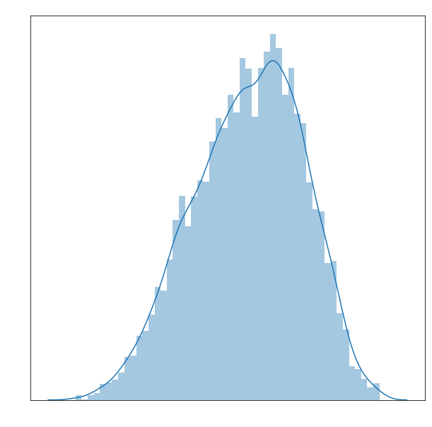
I did some exploration of the data distribution. First, it was interesting to see that Metacritic’s scores have a left skew. In general, the mean for a movie is around 75, which Metacritic should probably correct. I believe one way Metacritic addresses this discrapancy is by color coding their scores red, yellow, and green, with green starting at around a score of 65.
plt.figure(figsize=(10,10))
sns.distplot(Meta.Metascore, bins=50)
# plt.xlabel('Metascore', color='white')
# plt.title('Metascore Distribution', color='white')
# plt.tick_params(colors= 'white');
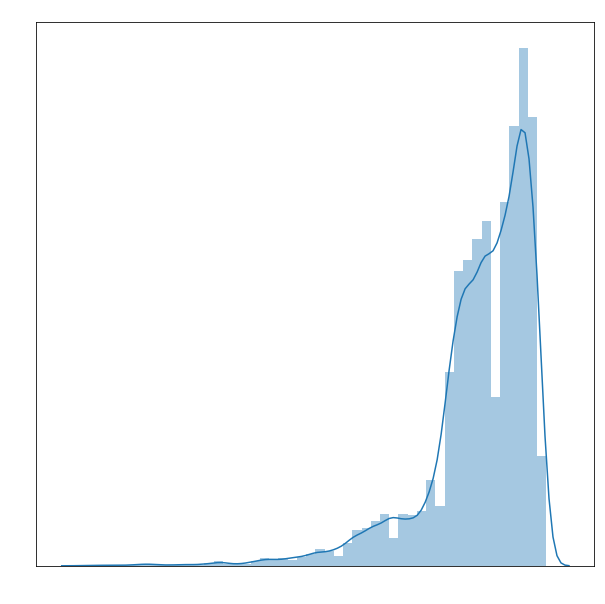
Another interesting fact is that the bulk of my Metacritic scores are from 2000 and after. This makes sense, as Metacritic was founded in 1999. (Source: https://en.wikipedia.org/wiki/Metacritic). Since then, they have retroactively scored old and popular films.
plt.figure(figsize=(10,10))
sns.distplot(Meta.Year, bins=50);
# plt.xlabel('Year Released', color='white')
# plt.title('Year Distribution', color='white')
# plt.tick_params(colors= 'white');
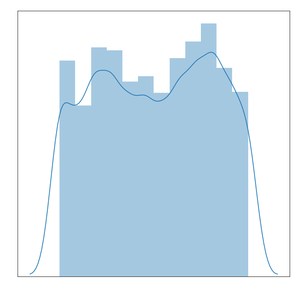
Here I looked at distribution by month of movies. There are bumps in the summer months as well as the fall months, as would be expected. Also, I see the month with the fewest movies released is February, which makes sense as that’s the month of the Academy Awards.
plt.figure(figsize=(10,10))
sns.distplot(Meta.month, bins=12);
# plt.xlabel('Month Released', color='white')
# plt.title('Month Distribution', color='white')
# plt.tick_params(colors= 'white');
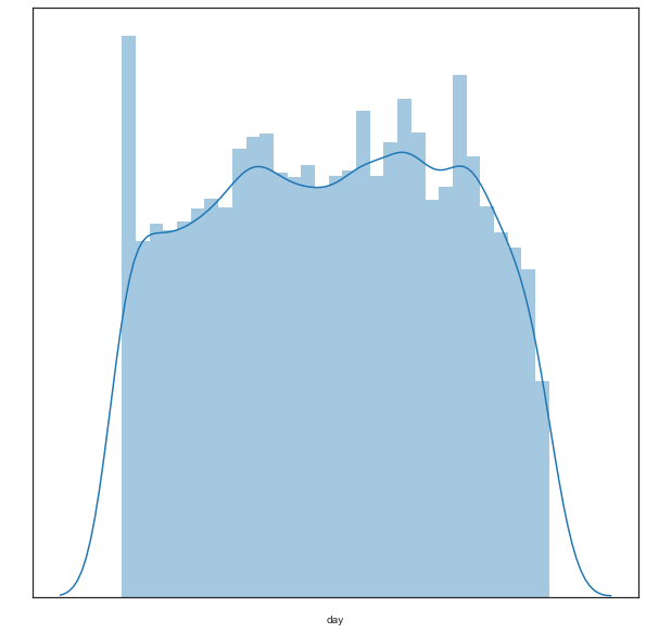
I looked at the distribution of movies by day of month, and although the plot is mostly uniform, it does tend to rise towards the end of the month. I do not konw the reason for this.
plt.figure(figsize=(10,10))
sns.distplot(Meta.day, bins=31);
# plt.xlabel('Day of Month Released', color='white')
# plt.title('Day Distribution', color='white')
# plt.tick_params(colors= 'white');
Meta.loc[9122,:]
Actors          Michèle Moretti|Hermine Karagheuz|Karen Puig|P...
Director                        Jacques Rivette|Suzanne Schiffman
Genre                                                       Drama
Metascore                                                      87
Production                                                Unknown
Rated                                                   NOT RATED
Runtime                                                       729
Title                                                       Out 1
Writer                                                        N/A
Year                                                         1971
imdbID                                                  tt0246135
imdbRating                                                    8.1
month                                                          11
day                                                            18
title_length                                                    5
Name: 9122, dtype: object
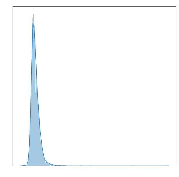
I looked at the distrbution of running time. As expected, most movies fall in between that 90 to 120 minute mark. There is a huge right skew to this graph because of two movies, one of which was 729 minutes long, called “Out 1.” (Source: https://en.wikipedia.org/wiki/Out_1). It’s actually a single movie divided into ten or so parts each of movie length. Critics say it’s one of the best movies ever made. I will have to take their word for it.
plt.figure(figsize=(10,10))
sns.distplot(Meta.Runtime, bins=240);
# plt.xlabel('Runtime', color='white')
# plt.title('Runtime Distribution', color='white')
# plt.tick_params(colors= 'white');
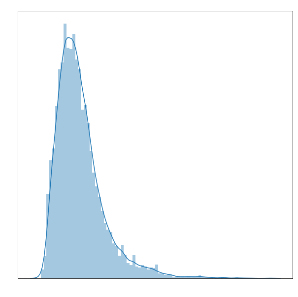
I looked at the distribution of length of title, and found that most movies are appromixatley 17 characters long. Not too illuminating, but that’s why they call it data exploration.
plt.figure(figsize=(10,10))
sns.distplot(Meta.title_length, bins=80);
# plt.xlabel('Length of Title', color='white')
# plt.title('Title Length Distribution', color='white')
# plt.tick_params(colors= 'white');
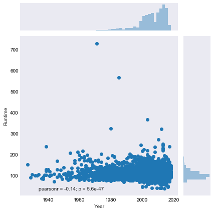
I plotted runtime by year as I have noticed movies getting longer on average in recent years and the data completely confirmed this.
# plt.figure(figsize=(10,10));
# sns.set_style("white",{"xtick.color":"white", "ytick.color":"white"})
sns.set_style("dark",{"xtick.color":"black", "ytick.color":"black"})

g = sns.jointplot(x="Year", y="Runtime", data=Meta)
# g.set_axis_labels(["x", "y"], color='white')
# g.fig.suptitle('Runtime vs. Year', color ='w');
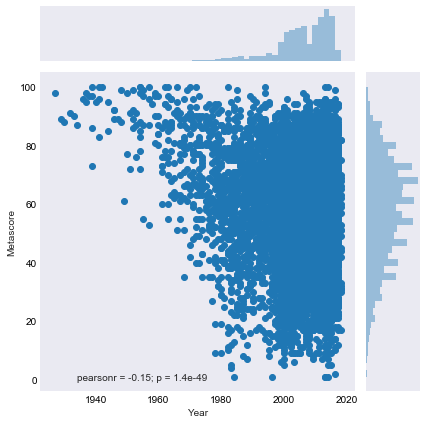
Here I plotted Metascore by year, but it wasn’t very illumating, except showing that the movies that Metacritic retroactively scored tended to be good movies, which makes sense.
plt.figure(figsize=(10,10))
# sns.set_style("white",{"xtick.color":"white", "ytick.color":"white"})
sns.set_style("dark",{"xtick.color":"black", "ytick.color":"black"})
g = sns.jointplot(x="Year", y="Metascore", data=Meta);
# g.set_axis_labels(["x", "y"], color='white')
# g.fig.suptitle('Metascore vs. Year', color ='w');
<matplotlib.figure.Figure at 0x1a15d1fc50>
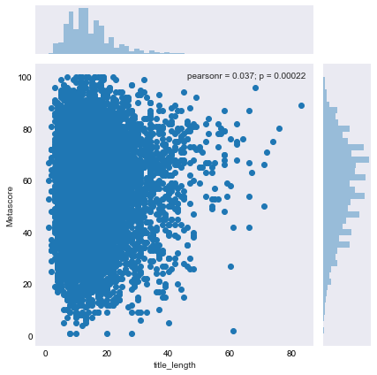
Then I plotted title length by score to see if there was any correlation. It is clear that movies who use longer titles are usually better, but that makes sense, considering the boldness and confidence required to give a movie a long title. If your’e going to give your movie a long title, you probably know the movie is going to be good. No one is wasting a long title on an Adam Sandler film.
sns.set_style("dark",{"xtick.color":"black", "ytick.color":"black"})
plt.figure(figsize=(10,10))
sns.jointplot(x="title_length", y="Metascore", data=Meta);
<matplotlib.figure.Figure at 0x1a15ddf9b0>
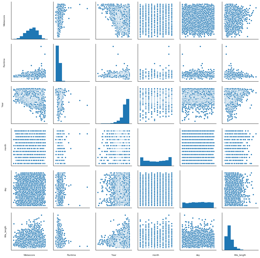
I generated a pairplot for the numerical values to see if any relationships jumped out, but none did. That said, this makes sense, as if there were clear relationhips they would be known and exploited already.
sns.pairplot(Meta.drop('imdbRating', axis=1))
After running a few models that performed poorly, I did a little feature engineering. I sought to weight the people involved in a movie by aggregating over their Metascores. To do this, I created three DataFrames where I isolated the directors, actors, and writers.
# Setting a custom train and test set

X_train = Meta.iloc[:9000,:]
X_test = Meta.iloc[9000:,:]


# Here I set Director, Actor, and Writer columns that got average scores over their movies

# Directors = Meta.iloc[:9000,:].drop(['Actors', 'Genre', 'Production', 'Rated',
#        'Runtime', 'Title', 'Writer', 'Year', 'imdbID', 'imdbRating', 'month', 'day',
#        'title_length'], axis=1)
# Actors = Meta.iloc[:9000,:].drop(['Director', 'Genre', 'Production', 'Rated',
#        'Runtime', 'Title', 'Writer', 'Year', 'imdbID', 'imdbRating', 'month', 'day',
#        'title_length'], axis=1)
# Writers = Meta.iloc[:9000,:].drop(['Actors', 'Genre', 'Production', 'Rated',
#        'Runtime', 'Title', 'Director', 'Year', 'imdbID', 'imdbRating', 'month', 'day',
#        'title_length'], axis=1)
X_train.columns
Index(['Actors', 'Director', 'Genre', 'Metascore', 'Production', 'Rated',
       'Runtime', 'Title', 'Writer', 'Year', 'imdbID', 'imdbRating', 'month',
       'day', 'title_length'],
      dtype='object')
I pulled out my list of actors by using a count vectorizer on my features to get lists of columns and aggregate over those lists. I found every director, actor, and writer’s mean Metascore.
# Using my custom split and join function to create three lists of train data directors actors and writers

# Directors, _ = movie_split_and_join(Directors, Directors, evan_train_test_df_cvec_capstone, 0)

# Actors, _ = movie_split_and_join(Actors, Actors, evan_train_test_df_cvec_capstone, 0)

# Writers, _ = movie_split_and_join(Writers, Writers, evan_train_test_df_cvec_capstone, 0)

# # Saving each director, actor, and writer in a data frame with their mean Metascore.

# directors_df = []
# for n in Directors.columns:
#     temp_tuple = (n, Directors[Directors[n]==1].Metascore.mean())
#     directors_df.append(temp_tuple)

# actors_df = []
# for n in Actors.columns:
#     temp_tuple = (n, Actors[Actors[n]==1].Metascore.mean())
#     actors_df.append(temp_tuple)

# writers_df = []
# for n in Writers.columns:
#     temp_tuple = (n, Writers[Writers[n]==1].Metascore.mean())
#     writers_df.append(temp_tuple)

# Saving each of my DataFrames as csvs for future use.

# pd.DataFrame(writers_df, columns=['name', 'avgscore']).to_csv('writers_df.csv',index=False)
# pd.DataFrame(actors_df, columns=['name', 'avgscore']).to_csv('actors_df.csv',index=False)
# pd.DataFrame(directors_df, columns=['name', 'avgscore']).to_csv('directors_df.csv',index=False)
ASIDE: The Average Actor Debacle
Originally, I tried to also replace the Actors column with an aggregate score for each member of the series of lists. For instance, if four people were listed in a movie, I’d take the average of their Metascores (their own average Metascore) and average that. Some actors wouldn’t have values or some movies might have no actors listed, so if I ran into those problems, I would just use an np.nan (Later, I would change this to a 666.666 to easily remove). Then I wouldn’t necessarily have to count vectorizer the Actors column. At first this seemed to have worked. It gave me better models (though only when I still count vectorized the Actors column). But this may have been a fluke. I noticed some of the data was strange looking. So I tried to reproduce the problem with my morta df.
# Beginnings of problems that plagued me

morta = df.dropna(axis=0, how='any', subset=['Metascore', 'imdbID']).copy()
morta['ActorAvg'] = 0.

# Here, for all actors in a movie, I add up their Metascores and average them.
# If the actors can't be found in actor df, that is, if they were only in movies without Metascores
# or were missed for whatever other reason, I assign a NaN value to the cell, to flag the row for later removal.

morta_list = []
for index, m in enumerate(morta.Actors):
    s=0
    den = 0
    for p in m:
        for n in zip(actors_df.name.values, actors_df.avgscore):
            if p.lower() == n[0]:
                s = s + n[1]
                den = den + 1
    if den == 0:
        morta.ActorAvg[index]=666.666
        morta_list.append(666.666)
    else:
        morta.ActorAvg[index]=s/den
        morta_list.append(s/den)
Morta was a copy of Meta that I applied my average program to. Unfortunately, when I tried to save my actor averages column, it was difficult to apply to the original data. Data seemed to disappear when I tried to link it with imdbid. I couldn’t get the column to sum consistently. WHen I told someone who knows more about python and pandas than I do, they told me I had discovered a bug. (I’m talking about you, Adam Blomberg!)
I dumped several hours into this so I’m going to leave the columns below intact as a testament to the madness this induced in me.
# morta.ActorAvg.sum()
6344793.712
# morta[['ActorAvg','imdbID']].sum()
ActorAvg                                                    0
imdbID      tt0017136tt0020269tt0020697tt0023634tt0024216t...
dtype: object
# morta['ActorAvg'].sum()
6344793.712
# morta['ActorAvg'].head()
17832      0.000
3026     666.666
23579      0.000
6808     666.666
18557      0.000
Name: ActorAvg, dtype: float64
# morta[['ActorAvg']].head()
| ActorAvg | |
|---|---|
| 17832 | 0.0 |
| 3026 | 0.0 |
| 23579 | 0.0 |
| 6808 | 0.0 |
| 18557 | 0.0 |
# morta.ActorAvg.sum()
6344793.712
# morta_df = pd.DataFrame(morta_list)
# pd.DataFrame(morta_list).to_csv('morta.csv', index=False, header=True)
# avgact = list(zip(morta.ActorAvg, morta.imdbID))
---------------------------------------------------------------------------

AttributeError                            Traceback (most recent call last)

<ipython-input-105-fa4907e8b3fe> in <module>()
----> 1 avgact = list(zip(morta.ActorAvg, morta.imdbID))


/anaconda3/lib/python3.6/site-packages/pandas/core/generic.py in __getattr__(self, name)
   3612             if name in self._info_axis:
   3613                 return self[name]
-> 3614             return object.__getattribute__(self, name)
   3615
   3616     def __setattr__(self, name, value):


AttributeError: 'DataFrame' object has no attribute 'ActorAvg'
# tempavg = []
# for m in avgact:
#     tempdic = {}
#     tempdic['ActorAvg'] = m[0]
#     tempdic['imdbID'] = m[1]
#     tempavg.append(tempdic)
# pd.DataFrame(tempavg).to_csv('NewActorAvg.csv', index=False, header=True)
# pd.DataFrame(tempavg).ActorAvg.sum()
187228.14293332995
# morta[['ActorAvg', 'imdbID']].to_csv('NewActorAvg.csv', index=False, header=True)
END OF ASIDE
Finally, I saved a few versions of of the DataFrame. One with directors weighted, one with directors and actors weighted, and one with direcotrs, actors, and writers weighted. Then for each of those I saved a version that was count vectorized only if a term appeared twice or if a term appeared three times. In total, six DataFrames to see which models the best.
X_train_to_concat, X_test_to_concat = movie_split_and_join(X_train.drop(['Director', 'Title', 'Actors', 'Writer'],
                                                                        axis=1),
                                                           X_test.drop(['Director', 'Title', 'Actors', 'Writer'],
                                                                       axis=1),
                                                                       evan_train_test_df_cvec_capstone,
                                                                       1)

title_train = X_train['Title']
title_test = X_test['Title']

director_train, director_test = single_column_cvec(X_train['Director'], X_test['Director'], 2)
actor_train, actor_test = single_column_cvec(X_train['Actors'], X_test['Actors'], 2)
writer_train, writer_test = single_column_cvec(X_train['Writer'], X_test['Writer'], 2)

cvec = CountVectorizer(binary=True,
                       stop_words = 'english',
                       strip_accents='unicode',
                       ngram_range = (1, 2))

cvec.fit(title_train)
lonely_matrix_train = cvec.transform(title_train)
lonely_matrix_test = cvec.transform(title_test)
title_train = pd.DataFrame(lonely_matrix_train.todense(), columns=cvec.get_feature_names())
title_test = pd.DataFrame(lonely_matrix_test.todense(), columns=cvec.get_feature_names())
director_train, director_test = put_in_avgs(director_train, director_test, directors_df)
X_train_direct = pd.concat([X_train_to_concat, title_train, director_train, writer_train, actor_train], axis=1)
X_test_direct = pd.concat([X_test_to_concat, title_test, director_test, writer_test, actor_test], axis=1)
# Saving my files to DataFrames with directors weighted

# pd.DataFrame(X_train_direct).to_csv('train_everything_director_weights_df2.csv')
# pd.DataFrame(X_test_direct).to_csv('test_everything_director_weights_df2.csv')
# pd.DataFrame(X_train_direct).to_csv('train_everything_director_weights_df3.csv')
# pd.DataFrame(X_test_direct).to_csv('test_everything_director_weights_df3.csv')
actor_train, actor_test = put_in_avgs(actor_train, actor_test, actors_df)
X_train_act = pd.concat([X_train_to_concat, title_train, director_train, writer_train, actor_train], axis=1)
X_test_act = pd.concat([X_test_to_concat, title_test, director_test, writer_test, actor_test], axis=1)
# Saving my files to DataFrames with directors and actors weighted

# pd.DataFrame(X_train_act).to_csv('train_everything_director_actor_weights_df2.csv')
# pd.DataFrame(X_test_act).to_csv('test_everything_director_actor_weights_df2.csv')
# pd.DataFrame(X_train_act).to_csv('train_everything_director_actor_weights_df3.csv')
# pd.DataFrame(X_test_act).to_csv('test_everything_director_actor_weights_df3.csv')
writer_train, writer_test = put_in_avgs(writer_train, writer_test, writers_df)
X_train_write = pd.concat([X_train_to_concat, title_train, director_train, writer_train, actor_train], axis=1)
X_test_write = pd.concat([X_test_to_concat, title_test, director_test, writer_test, actor_test], axis=1)
# Pre-made DataFrames with directors, actors, and writers weighted

# pd.DataFrame(X_train_write).to_csv('train_everything_director_actor_writer_weights_df2.csv')
# pd.DataFrame(X_test_write).to_csv('test_everything_director_actor_writer_weights_df2.csv')
# pd.DataFrame(X_train_write).to_csv('train_everything_director_actor_writer_weights_df3.csv')
# pd.DataFrame(X_test_write).to_csv('test_everything_director_actor_writer_weights_df3.csv')